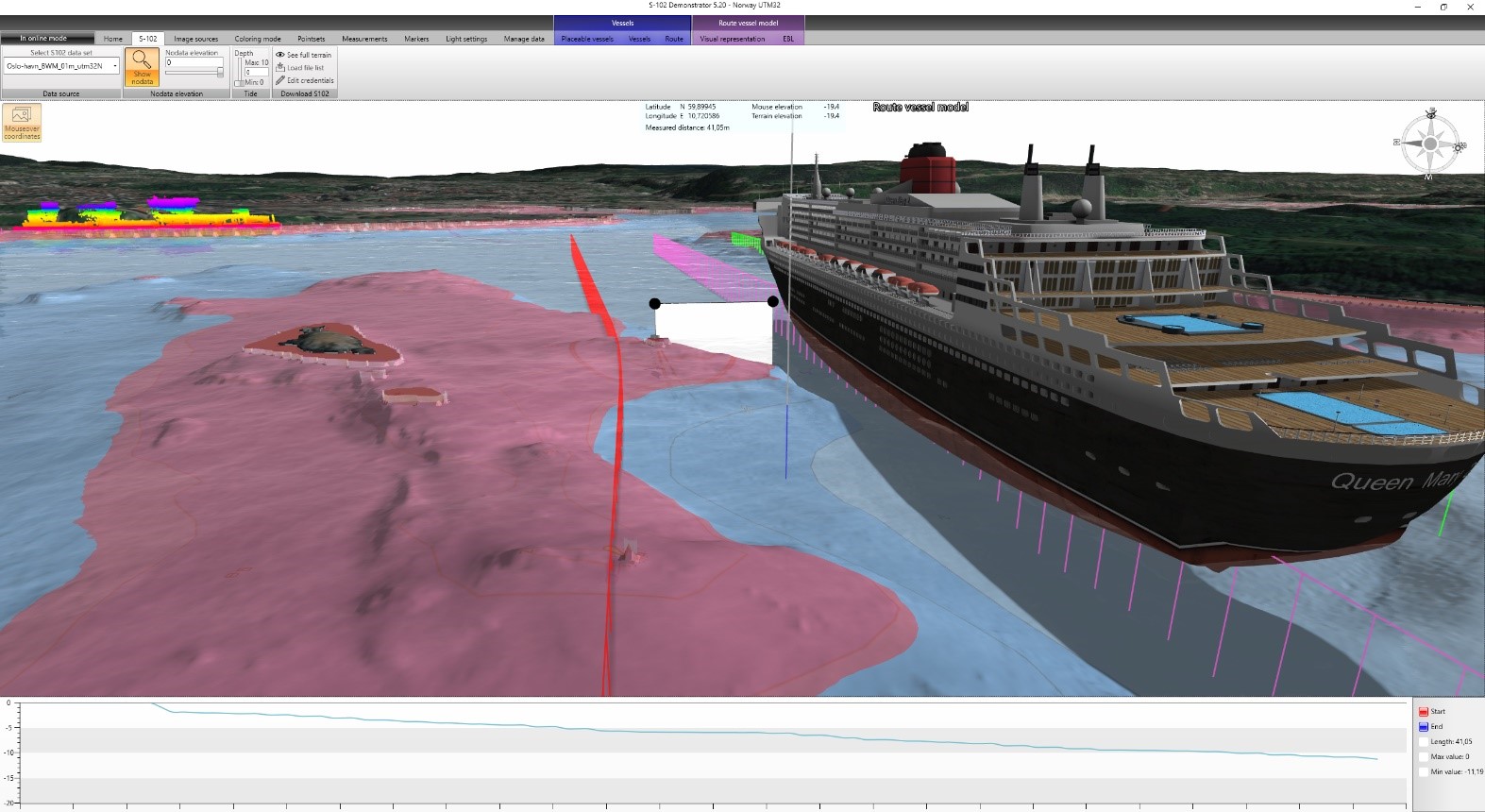
Relevant technical information related to S-102 visualisation tools
Kongsberg Digital has been responsible for the implementation of a demonstrator application in the research project. The goal of the application is to explore and demonstrate the possible uses for high resolution gridded bathymetry in the S-102 format.
Technical description of the demonstrator
The demonstrator has been implemented as a Windows desktop application, using the Microsoft WPF framework and the Kongsberg Cogs 3D visualisation toolbox. It has been deployed to end-users as a Windows Installer package, built using the WIX installer toolkit. These are well-known technologies for our development team and have enabled a very rapid turnaround cycle for new functionality and features. A future commercial product will most likely be based on a different platform such as tablet PC or even a web-based deployment, but exploring the details of such offerings was not in the scope of this project.
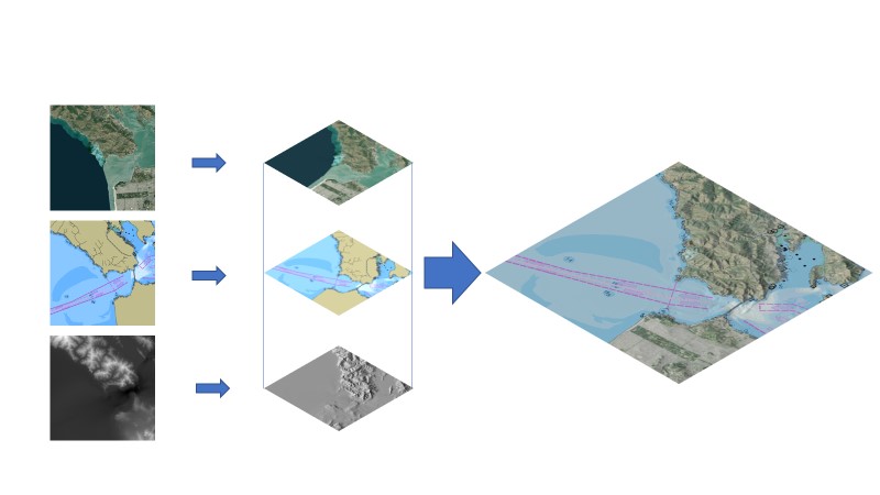
The Cogs 3D toolbox has a powerful terrain visualisation component which forms the basis of the demonstrator. It uses tile-based access to elevation and map data from online services, and dynamically builds an LOD (level-of-detail) pyramid of tiles in varying resolution, updating on-the-fly as the user navigates around in the 3D scene.
For this project, we are accessing elevation tiles for the bathymetry by reading subsets of the S-102 file, and land elevation tiles from the www.hoydedata.no web-service, using the ESRI ImageServer protocol. Additionally, we are accessing S57 map tiles from the ECC WMS service, as well as land imagery and topographic maps using the Statens Kartverk (Norwegian Mapping Authority) WMTS services.
For the moment, the demonstrator uses UTM (universal transverse mercator) projections exclusively. This is a system of 120 different projections, one for each 6-degree slice of the globe and for each hemisphere. For instance, mapping areas near Norway typically uses UTM zone 32 N or 33 N, whereas Canada might use zone 10 N or 18 N. The UTM projection has several properties making it very attractive for this sort of application:
- North is up
- Units are meters in all directions (no need to scale up or down)
- Preserves scale and shapes with little distortion
All of these properties are true only for areas close to the central meridian of the zone, so it is imperative to choose the correct zone for the work we want to do.
The demonstrator can, in theory, read data from virtually any projection, but internally it uses one UTM projection for everything. This means everything that is not stored or gridded in UTM will have to be reprojected in order to be shown in the demonstrator.
Every time map data is reprojected or resampled, it loses some information, depending on the resampling algorithm used, we typically lose either information about the magnitude of local minima or maxima (using smoothing algorithms such as bilinear or cubic), or the horizontal placement of the minima or maxima (using algorithms such as nearest neighbour or min/max).
To preserve as much information as possible about each grid cell, it is advised that the bathymetric grid itself is produced in UTM coordinates and that the same UTM grid for all surveys in one area.
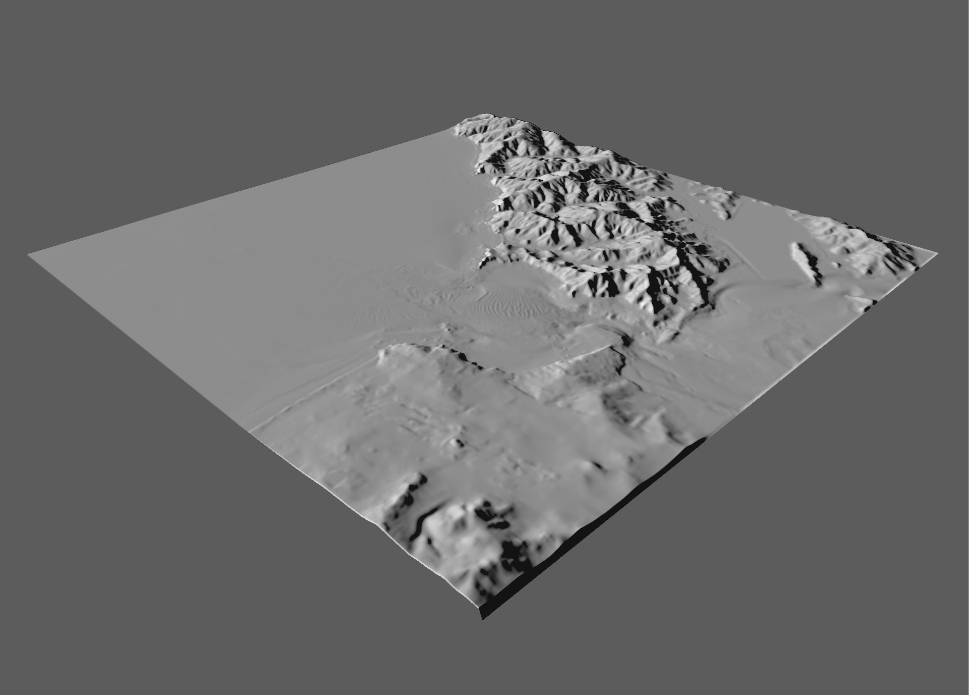
The demonstrator intends to manipulate the raw data as little as possible, as such we try to avoid all sorts of resampling and re-projection at the lowest level. However, since the demonstrator allows you to look at huge areas of data in the same view, we sometimes need to downsample the most distant data to a lower level of detail. When downsampling distant data we have been using cubic resampling for a compromise between smooth elevation terrain and preserving local extremes, but in the latest version we are transitioning to maximum value also for this resampling in order to preserve local maxima (shoalest depth) even when zoomed out.
We use elevation and bathymetry sources with different vertical datums but display them with the same origin value. For bathymetry data, the vertical datum used is typically based on “lowest astronomical tide”, giving depth values that are a bit more conservative than average, but for land elevation data the vertical datum used is typically “mean sea level”.
Land elevations are also clamped to minimum 1 meter to make a clearer distinction between land and bathymetry. When the user changes the tidal level, we only move the bathymetry data, keeping the land elevation and its relative sea level constant.
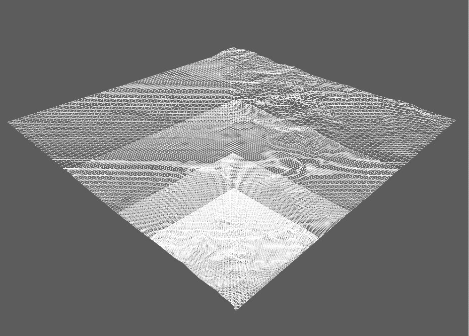
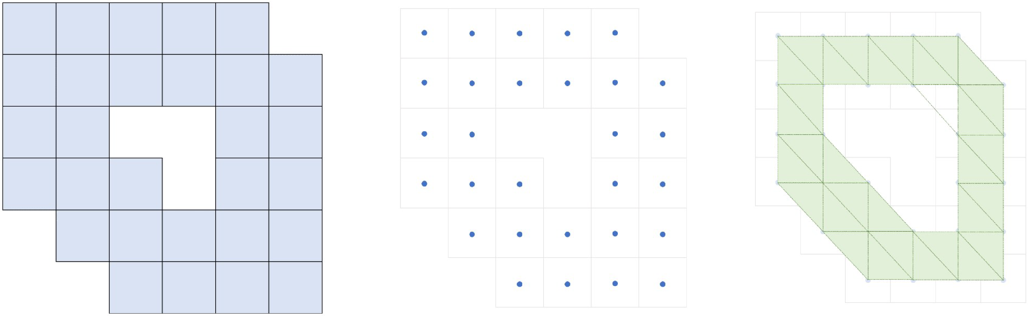
In order to visualise the elevation grid as a continuous surface, the terrain engine uses the horizontal center point of each grid cell and places a 3D vertex in that XY-position, using the elevation value as the Z-component of the position. Between pairs of neighbouring grid cells, the terrain engine places the edge of a triangle, such that 3 neighbour cells form one triangle in a triangle mesh, see the following top-down illustrations:
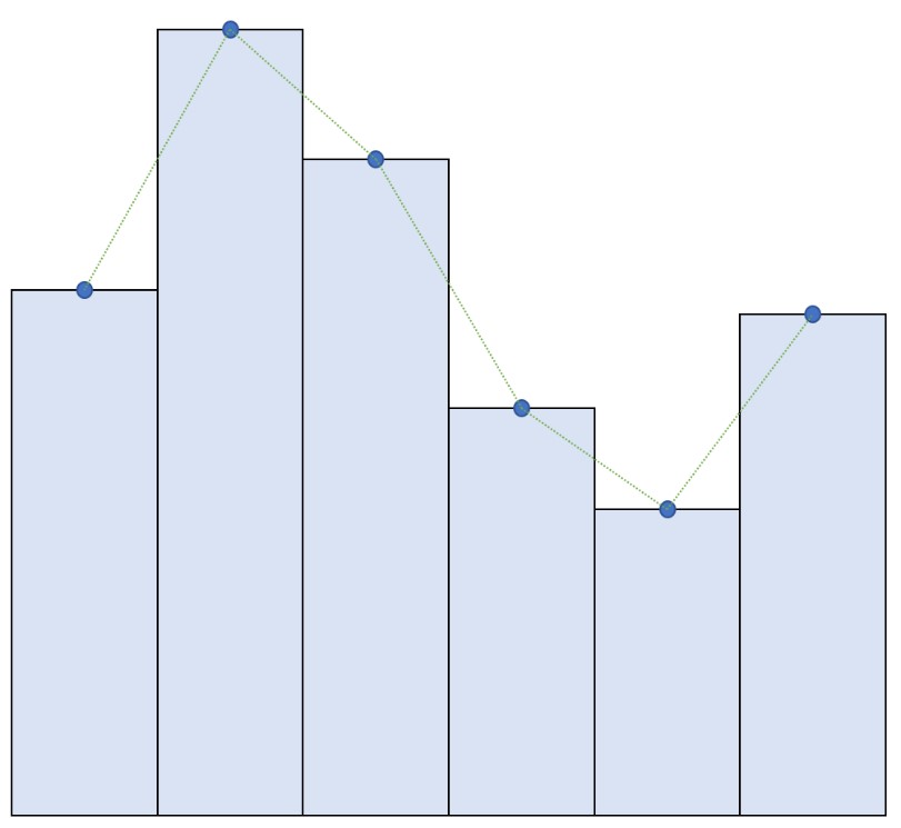
Since we let the cell centres be connected, this means that values between the center points of two neighbour cells will be linearly interpolated like in the following illustration (side view of a row of data from the grid):
For all calculations in the demonstrator we use the actual cell values for their entire extents, but for real-time visualisation purposes some areas will be represented as slightly deeper than the model gives any information about. This is a tradeoff between accuracy, performance and visual quality, and is only used in the real-time visualisation. As long as the grid itself is high resolution and produced with conservative depth values (using the “shoalest depth” algorithm for instance), this visualisation mode should be sufficient for most use cases. However, if an even more accurate (or pessimistic) representation should be desired it is possible to introduce that as a separate visualisation mode at a later point.
